The Science Behind
Axiorad
Standards-based RF propagation physics with explicit fidelity labels (validated / planning-grade / approximate / idealized). Multiple propagation models, an authoritative CPU-worker path, and multi-source DEM support. See methodology.
Every calculation traces back to a published standard or peer-reviewed reference. No proprietary black-box models — the physics are auditable, the assumptions are explicit, and the results are reproducible.
Five Propagation Models with Fidelity Labels
Five propagation models — including ITU-R and industry standards — cover a wide range of frequencies, distances, and environments. Automatic model selection evaluates each scenario's characteristics and applies the most appropriate physics. Not every model is an ITU-R Recommendation; see /methodology for labels.
Free-Space (Friis)
Any freq / distanceBaseline line-of-sight path loss for unobstructed propagation. Establishes the minimum possible path loss for a given frequency and distance.
Ref: Skolnik, Barton
Two-Ray Ground Reflection
< 10 kmCombines direct path with specularly reflected ground path. Models constructive and destructive interference patterns that dominate at short ranges.
Ref: Barton (2004)
COST-231 Hata
150–2000 MHz · 1–20 kmUrban and suburban empirical model extended from the Okumura-Hata formulation. ITU-R validated for land mobile systems in built-up environments.
Ref: ITU-R M.1225
Longley-Rice ITM
20 MHz–20 GHz · 1–2000 kmIrregular terrain model supporting LOS, diffraction, and troposcatter modes. Industry-standard model for wide-area coverage prediction over complex terrain.
Ref: Hufford et al. (1982)
ITU-R P.1812-6
30 MHz–6 GHzFull ITU standard path-specific propagation model. Incorporates Bullington diffraction, anomalous propagation, gaseous absorption, and location variability.
Ref: ITU-R P.1812-6
Line-of-Sight & Diffraction
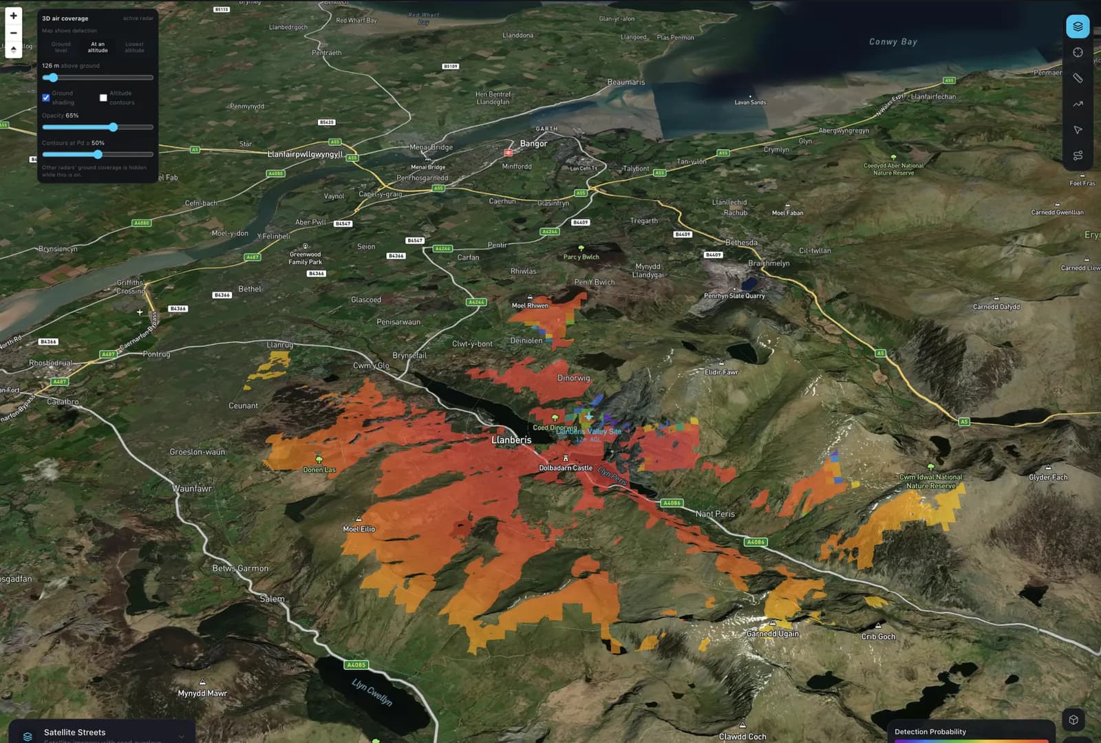
Line-of-sight analysis with Earth curvature correction, first Fresnel zone clearance checking, and ITU-R P.526 delta-Bullington diffraction for obstructed paths.
Earth Curvature & Atmospheric Refraction
Configurable k-factor (effective Earth radius multiplier) for atmospheric refraction. Presets: standard atmosphere (k = 4/3), no refraction (k = 1.0), super-refraction / ducting (k = 2.0). Surface refractivity (N₀) input derives k automatically. k-factor is propagated through all LOS, diffraction, clutter, and GPU calculations.
Fresnel Zone Clearance
First Fresnel zone radius computed along each path profile. Configurable clearance ratio (standard 60%) determines whether a path is LOS-clear or obstructed.
Bullington Terrain Diffraction
The whole terrain profile is reduced to one equivalent knife-edge (Bullington construction). Its Fresnel-Kirchhoff loss J(ν) follows ITU-R P.526, with the Recommendation's correction for multiple edges.
Delta-Bullington Smooth-Earth Term
ITU-R P.526-16 §4.5 adds spherical-Earth diffraction minus the Bullington loss of the smoothed profile, so long paths over curved terrain are not under-counted. The same module feeds the P.1812 fallback engine.
Antenna Pattern Import
Load measured or manufacturer-supplied patterns in Radio Mobile (.ant), MSI Planet (.msi/.pln), or two-column CSV/TSV format. Auto-detection identifies the format and interpolates sparse data to 1° resolution. Without an import, a 3GPP TR 38.901 parabolic beam is built from the beamwidths, with a 30 dB side-lobe floor.
Atmospheric, Rain & Vegetation Attenuation
Three ITU-R standard environmental models quantify signal degradation from atmospheric gases, precipitation, and vegetation.
Atmospheric Absorption
New CPU runs use P.676-13 Annex 1 line-by-line specific attenuation from O₂ and H₂O vapour over a homogeneous slant path with the supplied weather conditions. Below 1 GHz, the run records an explicitly identified legacy P.676-10 closed-form planning approximation as an extrapolation outside that method's documented 1–350 GHz domain. Critical at the 60 GHz oxygen resonance band and the 22 GHz water vapour absorption line. No field calibration or every-weather validation is implied.
Rain Attenuation
Specific attenuation γ = k·R^α with frequency and polarization-dependent coefficients from P.838-3. The active engine applies uniform specific attenuation across the slant path; non-uniform rain-cell reduction is not yet implemented.
Vegetation Loss
Weissberger model and the ITU-R saturation model for signal attenuation through woodland. Seasonal variation for deciduous trees — summer foliage adds 3–5 dB relative to winter bare-branch conditions.
Radar Detection Chain
Complete radar detection chain from the radar range equation through Swerling fluctuation models to detection probability. Two calculation methods are available: Albersheim's closed-form approximation for fast computation, and the Marcum Q-function for high-precision results at extreme P_d values.
Radar Range Equation
Pₜ = transmit power · Gₜ,Gᵣ = antenna gains · σ = target RCS · λ = wavelength · R = range · k = Boltzmann · Tₛ = system noise temp · B = bandwidth · L = system losses
Swerling Fluctuation Models
Five target models (Swerling 0–4) covering steady, scan-to-scan, and pulse-to-pulse RCS fluctuation statistics. Target type selection affects the required SNR for a given detection probability.
Detection Probability
v1.10.0Two detection models are available. Albersheim's approximation (default) converts SNR, number of pulses integrated, and required P_fa to P_d via a fast closed-form expression. The Marcum Q-function uses numerical integration (Rice integral with Bessel I₀ approximation) for higher accuracy at extreme P_d values (< 0.1 or > 0.99). Both support Swerling 0–4 fluctuation statistics.
Firm Track Probability
v1.1.0M-out-of-N binomial model for track initiation probability. Computes the probability that a target generates M or more detections out of N consecutive scans — a common track initiation criterion (e.g. 2-of-3, 3-of-5).
Vertical Coverage (Blake Chart)
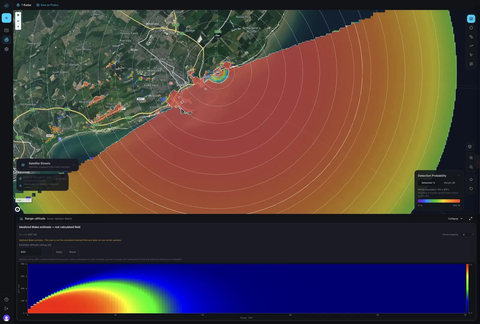
v1.4.0Range vs. altitude analysis reveals detection probability contours across the vertical coverage envelope. Shows multipath nulls, beam elevation limits, and coverage holes — essential for siting studies and engagement geometry planning.
Pd heatmap
Color-coded 2D grid (range × altitude)
Contour lines
50% and 90% Pd threshold overlays
SCNR mode
Clutter-limited when clutter modeling active
Interactive panel
Floating, minimizable chart panel
Antenna Pattern Modeling
v1.5.0Import measured or manufacturer-supplied antenna patterns in multiple industry formats. The engine applies the loaded pattern to the radar equation gain term, replacing the default Gaussian beam approximation with real directional data.
Two-column import
CSV, TSV, or space-delimited angle/gain pairs
MSI/Planet format
Industry-standard .msi and .pln file support
Auto-detection
Format, plane (az/el), and delimiter detected automatically
Interpolation
Sparse patterns interpolated to 1° resolution; Gaussian fallback
Clutter Modeling
v1.3.0Real-world radar detection is limited by clutter — unwanted returns from the ground, sea, and precipitation. The SCNR (Signal-to-Clutter+Noise Ratio) model combines thermal noise with surface and volume clutter to compute realistic detection probability.
Land surface clutter
Constant-gamma model with grazing-angle-dependent reflectivity. Configurable surface types: rural, urban, forest, custom.
Sea surface clutter
Georgia Institute of Technology (GIT) model, valid 1–100 GHz. Incorporates wind speed, sea state, and polarization effects.
Rain volume clutter
Backscatter via Marshall-Palmer Z-R relationship (Z = 200·R^1.6). Clutter cell volume determined by range resolution and beam geometry.
SCNR visualization
SCNR map mode replaces SNR when clutter is active. Range resolution parameter controls clutter cell area computation.
ECM Resilience Analysis
v1.7.0Models noise jamming effects on radar detection. Stand-off jammers at fixed positions enter through antenna sidelobes; self-screening jammers on the target enter through the mainlobe. Supports barrage (wideband) and responsive (narrowband) modes with burn-through range calculation.
Stand-off jammer
Fixed-position jammer at a configurable lat/lon and altitude. Jamming power enters via antenna sidelobes; constant power across all target cells.
Self-screening jammer
Target-mounted jammer entering through the radar mainlobe. Jamming power scales with range² (one-way path), producing a range-dependent burn-through threshold.
Barrage / responsive modes
Barrage mode spreads power across the full radar bandwidth. Responsive mode concentrates power in the radar's instantaneous bandwidth, increasing effective jamming density.
S/(N+C+J) detection
Jamming power is summed with thermal noise and clutter in the interference denominator. Detection probability is computed from the composite SCNJ ratio.
Sensitivity Time Control (STC)
v1.8.0STC reduces receiver gain at close range to prevent saturation from strong clutter returns. The gain ramps back up as range increases, restoring full sensitivity beyond the configured STC range limit.
k = attenuation law exponent (2 = R², 3 = R³, 4 = R⁴). Applied as an SNR penalty before detection probability calculation.
Signal Processing
v1.9.0Waveform-based processing gain replaces the flat gain assumption with physically-derived values computed from pulse width, pulse repetition frequency, and compression ratio. Coherent integration accumulates energy phase-coherently; non-coherent integration models the square-root gain of envelope detection. Simple mode retains a single flat processing gain input for quick estimates.
Pulse compression gain
G_pc = 10·log₁₀(τ·B_w) dB, where τ is pulse width and B_w is waveform bandwidth. Derived from time-bandwidth product.
Coherent integration
G_int = 10·log₁₀(N) dB — full N-pulse coherent gain. Requires phase stability across the dwell; applicable to pulsed-Doppler waveforms.
Non-coherent integration
G_int ≈ 10·log₁₀(N^0.5) dB — square-root gain from envelope detection of N independent pulses. Conservative estimate for incoherent receivers.
Unambiguous range & blind velocity
R_ua = c / (2·PRF). Blind velocity v_b = λ·PRF / 2. Both derived from PRF; displayed as waveform performance metrics alongside processing gain.
Total processing gain = pulse compression gain + integration gain. Applied additively (dB) to the SNR from the radar range equation before detection probability is computed.
Authoritative CPU Worker
Coverage runs use the browser CPU worker so the selected propagation, detector, clutter, and result-metric contracts are applied consistently. An experimental WebGL kernel remains in the codebase for research, but it is not used for authoritative analysis runs.
Grid Generation
A polar-to-Cartesian coverage grid is generated at configurable resolution. Each cell represents a geographic point to be evaluated. Grid density is balanced against render performance.
Per-Cell Evaluation
The CPU worker evaluates each grid cell with the selected terrain, propagation, environmental, detector, and output-metric configuration. Work is kept off the main UI thread.
Float32 Output
Results are written to typed arrays containing the calculated metrics and coverage state, then transferred from the worker to the Deck.gl rendering layer.
Experimental GPU Kernel Status
The CPU worker is the authoritative calculation path. A simplified WebGL kernel remains available to developers for parity research, but it does not yet implement the complete detector, environmental, clutter, and output-metric contract and is therefore not used for authoritative analysis runs.
Digital Elevation Model Sources
Multi-source digital elevation model support with automatic fallback. Choose the source that best fits your accuracy and coverage requirements.
| Source | Resolution | Coverage | Type |
|---|---|---|---|
| SRTM | 30 m / 90 m | Global (±60° lat) | Free |
| Mapbox Terrain | ~30 m | Global | API |
| Google Elevation | ~30 m | Global | API |
| OpenElevation | ~30 m | Global | Free API |
Elevation sources are queried per-tile as the analysis area is defined. If the primary source is unavailable, the engine automatically falls back to the next configured source. SRTM tiles are served from Axiorad's own CDN for consistent performance without requiring a Google or Mapbox API key.
Start your coverage study
Ready to analyze?
Open the Axiorad analyser and apply these physics to your own radar scenario — no installation required.
Planning-grade models · explicit fidelity labels · see /methodology